Modeling the vibrational behavior in a isotropic model of the tympanic membrane.
The tympanic membrane is a structure that resides in our ear. The behavior of that little membrane can be modeled by the wave equation:
\begin{equation} \frac{\partial^2 u}{\partial t^2}=c^2\frac{\partial^2u}{\partial x^2} \end{equation}
This equation will be constrained by the values:
\begin{equation} 0<x<l\hspace{2mm} \land\hspace{2mm} 0<t<t_f \end{equation}
The boundary conditions of our system will be:
\begin{equation} u(0,t)=u(l,t)=0 \hspace{2mm} \end{equation}
And the initial conditions are:
\begin{equation} \frac{\partial u_x^0}{\partial t}=0 \hspace{2mm}\land\hspace{2mm} u(x,0)=sin(\frac{n\pi x}{L}) \end{equation}
Where $n$ is the vibrational mode. The values are $n=1,2,3,\cdots$ but I’m gonna observe only the first five vibrational node.
The values that we can use are:
- $L_T=4x10^{-5}m$ that is the large of the tense part.
- $L_f=1x10^{-4}m$ that is the large of the flacid part.
- $t_0=0$
- $t_f=2.42x10^{-7}s$
- $E=2x10^7Pa$
- $\rho_T=1000kg/m^3$ being the density of the tense part.
- $\rho_f=1200kg/m^3$ being the density of the flacid part.
- $\mu=0.3$ being the Poison module.
In this case, the propagation velocity $(c)$ is:
\begin{equation} c=\sqrt{\frac{E}{\rho}\frac{(1-\mu)}{((1+\mu)(1-2\mu))}} \end{equation}
I’m gonna use finite difference to solve the PDE. I will use the following libraries.
%matplotlib inline
import numpy as np
import pandas as pd
import matplotlib.pyplot as plt
from matplotlib.animation import FuncAnimation
from numba import njit
from jupyterthemes import jtplot
jtplot.style(theme='monokai')
If you’re wondering, what is Numba? It’s a library of Python that makes the codes a lot more fast than before. This can let us run a code in $10ms$ when before the codes run in $5s$. If you want to get more into this, you can check here.
I need to create all the variables i had to use.
lt=4e-5
lf=1e-4
tf=2.42e-7
E=2e7
rhot=1000
rhof=1200
mu=0.3

#Now, create the variable c
ct=np.sqrt((E/rhot)*((1-mu)/((1+mu)*(1-2*mu))))
cf=np.sqrt((E/rhof)*((1-mu)/((1+mu)*(1-2*mu))))

#Now, choose the number of grid points
Nx=551
Nt=551
dxt=(lt)/(Nx-1)
dxf=(lf)/(Nx-1)
dt=(tf)/(Nt-1)

#Create the arrays for x and t
xt=np.linspace(0,lt,Nx)
xf=np.linspace(0,lf,Nx)
t=np.linspace(0,tf,Nt)

@njit() #Create a function that calculates the cfl condition
def cfl(c,dt,dx):
    return c*(dt/dx)

#Use it to calculate the CFL condition
kt=cfl(ct,dt,dxt)
kf=cfl(cf,dt,dxf)

print('''The CFL condition is
kt={f}
kf={d}'''.format(f=kt,d=kf))
That says me that $k_f=0.362$ and $k_t=0.99$. Both criterion are good so we can follow.
Now, it’s time to make to use Finite Difference with our equation. The discretized derivates are:
\begin{equation} \frac{\partial^2 u}{\partial x^2}\approx\frac{u_{x+1}^{t}-2u_{x}^{t}+u_{x-1}^{t}}{\Delta x^2} \end{equation}
\begin{equation} \frac{\partial^2 u}{\partial t^2}\approx\frac{u_{x}^{t+1}-2u_{x}^{t}+u_{x}^{t-1}}{\Delta t^2} \end{equation}
The discretized equation is:
\begin{equation} \frac{u_{x}^{t+1}-2u_{x}^{t}+u_{x}^{t-1}}{\Delta t^2}=c^2\frac{u_{x+1}^{t}-2u_{x}^{t}+u_{x-1}^{t}}{\Delta x^2} \end{equation}
Now, we can use some algebra and get the next equation:
\begin{equation} u_x^{t+1}=k^2(u_{x+1}^{t}+u_{x-1}^{t})+2u_{x}^{t}(1-k^2)-u_x^{t-1} \end{equation}
where $k=c\frac{dt}{dx}$.
This equation can now be programmed. But first, we need to check the first time step so we can calculate $u_x^2$ using $u_x^1$ and $u_x^0$. That means:
\begin{equation} u_x^1=k^2(u_{x+1}^{0}+u_{x-1}^{0})+2u_{x}^{0}(1-k^2)-u_x^{-1} \end{equation}
We don’t know $u_x^{-1}$, that’s outside our time domain and our time mesh, how we can calculate? Well, we can calculate the discretized form our a first time derivate, that means:
\begin{equation} \frac{\partial u_x^{0}}{\partial t}\approx\frac{u_x^1-u_x^{-1}}{2\Delta t} \end{equation}
We know that from our initial conditions, we can get $\frac{\partial u_x^0}{\partial t}=0$. So we have:
\begin{equation} u_x^{-1}=u_x^1 \end{equation}
So, back to our equation to calculate $u_x^1$, we have:
\begin{equation} u_x^1=\frac{1}{2}k^2(u_{x+1}^{0}+u_{x-1}^{0})+u_{x}^{0}(1-k^2) \end{equation}
Now, we have everything that we need for compute the solution.
Thanks to the book Finite Difference Computing with PDEs written by Hans Petter Langtangen and Svein Linge.
I create three functions to solve this PDE. One is where I used the finite difference method. That is:
@njit() #Function to execute finite difference method
def fdm(Nx,Nt,l,tf,k,x,t,n):
    u=np.zeros((Nx,Nt))
    u=BC(u,l,Nx,Nt) #First, we initialize the BC
    u=IC(u,Nt,Nx,x,k,n,l) #And nowm we calculate the IC

    for j in range(1,Nt-1):
        for i in range(Nx-1):
            u[i,j+1]=k**2*(u[i+1,j]+u[i-1,j])+2*u[i,j]*(1-k**2)-u[i,j-1]
        u=BC(u,l,Nx,Nt)
    return u
Also, I use another to put the initial condition on my solution matrix.
@njit() #With this, we can calculate the initial conditions
def IC(u,Nt,Nx,x,k,n,l):
    for j in range(1,Nx-2):
        u[j,0]=np.sin(n*np.pi*x[j]/l)
        #u[j,0]=np.sin(np.pi*x[i])+0.5*np.sin(3*np.pi*x[i])
    for i in range(Nx-1):
        u[i,1]=0.5*k**2*(u[i+1,0]+u[i-1,0])+u[i,0]*(1-k**2)
    return u
And for last, I create a function that impose the boundary conditions.
@njit() #This is for the boundary conditions
def BC(u,l,Nx,Nt):
    for j in range(Nt-1):
        u[0,j]=0
        u[Nx-1,j]=0
    return u
After that, I can solve the equation for different $n$. The graph of the solution of the system are:
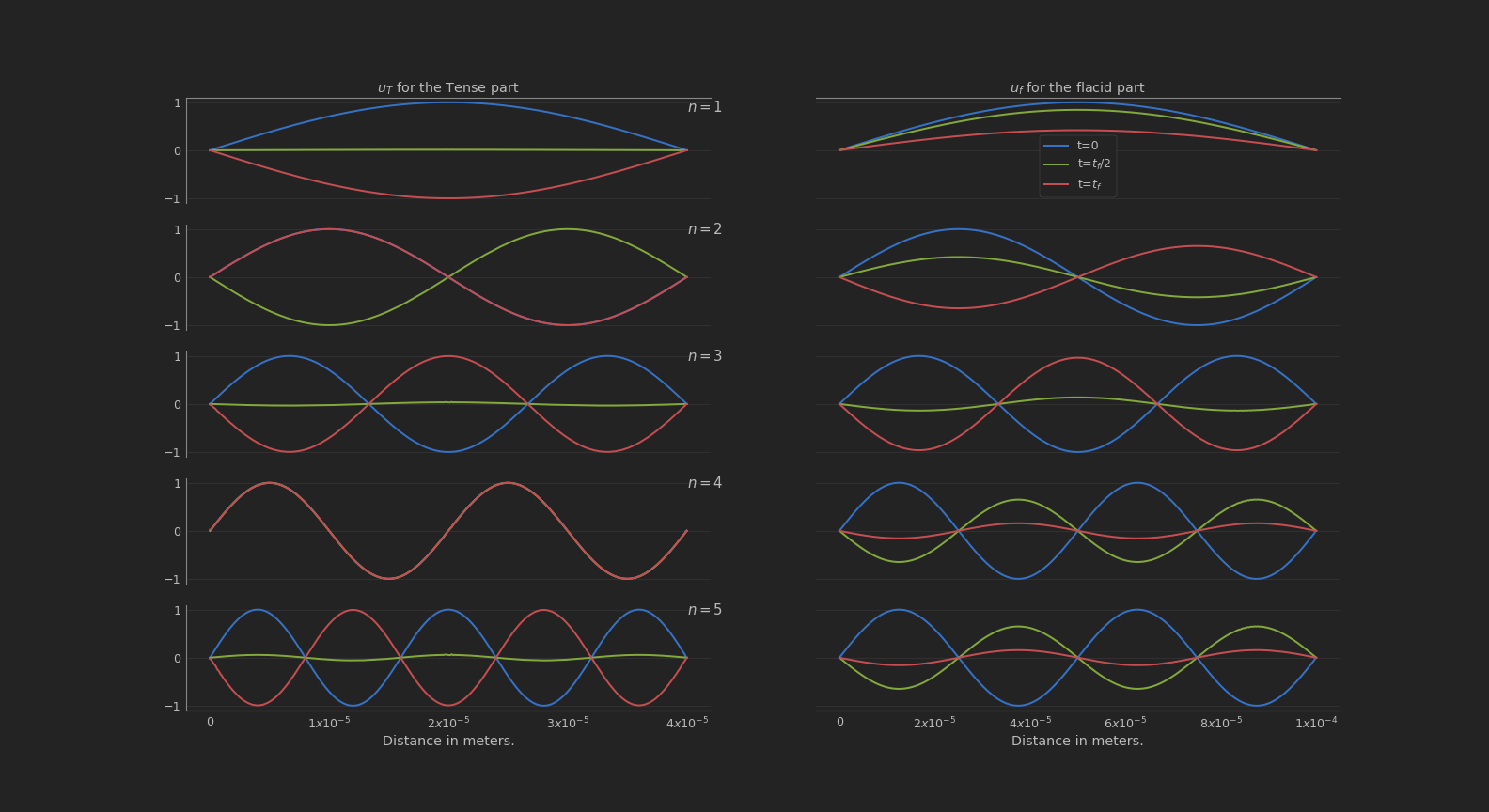
I only check the initial time, that is when $t=0$, also the middle time, that is when $t=\frac{t_f}{2}$ and the final time $t=t_f$.
To give a more clean view of the entire system at all timesteps, i create a video.
We can observe that both part have a similar movement. It’s also easy to see that the flacid part have a movement problem and can’t follow the rhythm of the tense part.
That’s all for this post! You can check the jupyter notebook from this problem here.