North america change in temperature
In this project, I decide to make a comparison in North America to check the $CO_2$ emittions and the temperature change between the years. In particular, I’m gonna work with United States, Canada and Mexico. I’m gonna check how many $CO_2$ produce every country from 1960 until now, and also check the average temperature.
First, let me import the libraries to use
import numpy as np
import matplotlib.pyplot as plt
import pandas as pd
import jupyterthemes as jtplot
from jupyterthemes import jtplot
jtplot.style(theme='monokai')
Now, I need to open the datasets.
data1=pd.read_csv('temperature.csv',skiprows=4)
data2=pd.read_csv('API_EN.ATM.CO2E.PC_DS2_en_csv_v2_1927797.csv',skiprows=3)
data3=pd.read_csv('mexico.csv',header=None,skiprows=1)
data4=pd.read_csv('canada.csv',header=None,skiprows=1)

usa_temp=pd.DataFrame(data1)
CO2=pd.DataFrame(data2)
mexico_temp=pd.DataFrame(data3)
canada_temp=pd.DataFrame(data4)

min_year=1960 #It's an arbitrary value
Work with the first data set. The USA temperature. Let’s check the data
usa_temp.head()
| Date | Value | Anomaly | |
|---|---|---|---|
| 0 | 196012 | 51.44 | -0.58 |
| 1 | 196112 | 51.87 | -0.15 |
| 2 | 196212 | 51.9 | -0.12 |
| 3 | 196312 | 52.26 | 0.24 |
| 4 | 196412 | 51.67 | -0.35 |
The best thing I can do it’s to change the name of the columns and also quit the column Anomaly, that because isn’t work for my analysis.
usa_temp=usa_temp.rename(columns={'Date':'Year',
                                  'Value':'Temperature'}).drop(columns='Anomaly')
def celsius_to_fah(x):
    return (x*(9/5))+32

def fah_to_celsius(x):
    return (x-32)*(5/9)

for i in range(len(usa_temp)):
    usa_temp['Year'][i]=min_year+i
    usa_temp['Temperature'][i]=fah_to_celsius(usa_temp['Temperature'][i])
usa_temp.head()
| Year | Temperature | |
|---|---|---|
| 0 | 1960 | 10.8 |
| 1 | 1961 | 11.0389 |
| 2 | 1962 | 11.0556 |
| 3 | 1963 | 11.2556 |
| 4 | 1964 | 10.9278 |
I want the change of the temperature, I mean i want the $\Delta T$. This differential it can be calculated by $\Delta T=T_i-T_0$, where $T_i$ is the actual temperature and $T_0$ is the initial temperature, at the year 1960. I’m going to create a new column with this $\Delta T$
dT=[]
#dT.append(0)
T0=usa_temp['Temperature'][0]
for i in range(1,len(usa_temp)):
    dT.append(usa_temp['Temperature'][i]-T0)

usa_temp=usa_temp.join(pd.DataFrame({'dT':dT}))
usa_temp.head()
| Year | Temperature | $\Delta T$ | |
|---|---|---|---|
| 0 | 1960 | 10.8 | 0.238889 |
| 1 | 1961 | 11.0389 | 0.255556 |
| 2 | 1962 | 11.0556 | 0.455556 |
| 3 | 1963 | 11.2556 | 0.127778 |
| 4 | 1964 | 10.9278 | 0.138889 |
Now, It’s time to work with the data from Mexico.
mexico_temp=mexico_temp.rename(columns={0:'Temperature',1:'Year',
                                        2:'Statistics',3:'Country',4:'ISO3'})
mexico_temp.head()
| Temperature | Year | Statistics | Country | ISO3 | |
|---|---|---|---|---|---|
| 0 | 15.5146 | 1901 | Jan Average | Mexico | MEX |
| 1 | 15.3109 | 1901 | Feb Average | Mexico | MEX |
| 2 | 17.8516 | 1901 | Mar Average | Mexico | MEX |
| 3 | 19.6372 | 1901 | Apr Average | Mexico | MEX |
| 4 | 22.5504 | 1901 | May Average | Mexico | MEX |
Okey, i’ll manipulate the data to drop some columns and add the $\Delta T$ column
mexico_temp=mexico_temp.drop(columns={'Statistics','Country','ISO3'})
mexico_temp=mexico_temp.where(mexico_temp['Year']>=min_year).dropna()
mexico_temp=mexico_temp.groupby('Year').mean().reset_index()
mexico_temp['Year']=mexico_temp['Year'].astype('int')

#I'm also add the dT column.
dT=[]
#dT.append(0)
T0=mexico_temp['Temperature'][0]
for i in range(len(mexico_temp)):
    dT.append(mexico_temp['Temperature'][i]-T0)
mexico_temp=mexico_temp.join(pd.DataFrame({'dT':dT}))
mexico_temp.head()
| Year | Temperature | $\Delta T$ | |
|---|---|---|---|
| 0 | 1960 | 20.509 | 0 |
| 1 | 1961 | 20.4919 | -0.01705 |
| 2 | 1962 | 20.838 | 0.32905 |
| 3 | 1963 | 20.6835 | 0.1745 |
| 4 | 1964 | 20.3534 | -0.155592 |
Now it’s time to clean the Canada data.
canada_temp=canada_temp.rename(columns={0:'Temperature',1:'Year',2:'Statistics',
                                        3:'Country',4:'ISO3'})
canada_temp.head()
| Temperature | Year | Statistics | Country | ISO3 | |
|---|---|---|---|---|---|
| 0 | -25.385 | 1901 | Jan Average | Canada | CAN |
| 1 | -23.719 | 1901 | Feb Average | Canada | CAN |
| 2 | -18.934 | 1901 | Mar Average | Canada | CAN |
| 3 | -9.9643 | 1901 | Apr Average | Canada | CAN |
| 4 | 0.02289 | 1901 | May Average | Canada | CAN |
Just like i did with Mexico, i am gonna do the same with Canada.
canada_temp=canada_temp.drop(columns={'Statistics','Country','ISO3'})
canada_temp=canada_temp.where(canada_temp['Year']>=min_year).dropna()
canada_temp=canada_temp.groupby('Year').mean().reset_index()
canada_temp['Year']=canada_temp['Year'].astype('int')
#I'm also add the dT column.
dT=[]
#dT.append(0)
T0=canada_temp['Temperature'][0]
for i in range(len(canada_temp)):
    dT.append(canada_temp['Temperature'][i]-T0)
canada_temp=canada_temp.join(pd.DataFrame({'dT':dT}))
canada_temp.head()
| Year | Temperature | $\Delta T$ | |
|---|---|---|---|
| 0 | 1960 | -6.4908 | 0 |
| 1 | 1961 | -7.39057 | -0.899773 |
| 2 | 1962 | -6.97667 | -0.485867 |
| 3 | 1963 | -6.79263 | -0.301832 |
| 4 | 1964 | -7.67968 | -1.18888 |
And for last, it’s time to clean the CO2 data from every coutry.
#Check the data
CO2.head()
| Country Name | Country Code | Indicator Name | Indicator Code | 1960 | 1961 | 1962 | 1963 | 1964 | 1965 | 1966 | 1967 | 1968 | 1969 | 1970 | 1971 | 1972 | 1973 | 1974 | 1975 | 1976 | 1977 | 1978 | 1979 | 1980 | 1981 | 1982 | 1983 | 1984 | 1985 | 1986 | 1987 | 1988 | 1989 | 1990 | 1991 | 1992 | 1993 | 1994 | 1995 | 1996 | 1997 | 1998 | 1999 | 2000 | 2001 | 2002 | 2003 | 2004 | 2005 | 2006 | 2007 | 2008 | 2009 | 2010 | 2011 | 2012 | 2013 | 2014 | 2015 | 2016 | 2017 | 2018 | 2019 | 2020 | Unnamed: 65 | |
|---|---|---|---|---|---|---|---|---|---|---|---|---|---|---|---|---|---|---|---|---|---|---|---|---|---|---|---|---|---|---|---|---|---|---|---|---|---|---|---|---|---|---|---|---|---|---|---|---|---|---|---|---|---|---|---|---|---|---|---|---|---|---|---|---|---|---|
| 0 | Aruba | ABW | CO2 emissions (metric tons per capita) | EN.ATM.CO2E.PC | 204.62 | 208.823 | 226.118 | 214.8 | 207.616 | 185.204 | 172.12 | 210.779 | 194.887 | 253.579 | 281.996 | 243.87 | 234.887 | 258.82 | 233.489 | 168.729 | 360.853 | 189.163 | 161.804 | 170.083 | 174.698 | 165.105 | 182.259 | 92.381 | 228.356 | 266.475 | 2.86832 | 7.2352 | 10.0262 | 10.6347 | 7.84745 | 8.22808 | 7.89989 | 8.95204 | 8.60574 | 8.81095 | 8.72675 | 8.88309 | 9.24344 | 9.10519 | 26.1949 | 25.934 | 25.6712 | 26.4205 | 26.5173 | 27.2007 | 26.9477 | 27.895 | 26.2296 | 25.9153 | 24.6705 | 24.5075 | 13.1577 | 8.35356 | 8.41006 | 8.61037 | 8.42691 | nan | nan | nan | nan | nan |
| 1 | Afghanistan | AFG | CO2 emissions (metric tons per capita) | EN.ATM.CO2E.PC | 0.0460567 | 0.0535888 | 0.0737208 | 0.0741607 | 0.0861736 | 0.101285 | 0.107399 | 0.12341 | 0.115142 | 0.0865099 | 0.149651 | 0.165208 | 0.129996 | 0.135367 | 0.154503 | 0.167612 | 0.153558 | 0.181522 | 0.161894 | 0.167066 | 0.131783 | 0.150615 | 0.163104 | 0.201224 | 0.231961 | 0.293957 | 0.267772 | 0.26923 | 0.246823 | 0.233882 | 0.210643 | 0.183364 | 0.0961966 | 0.0850871 | 0.0758065 | 0.0686399 | 0.0624346 | 0.0566423 | 0.0527632 | 0.0407225 | 0.0372348 | 0.0378461 | 0.0473773 | 0.0512556 | 0.0370753 | 0.051744 | 0.0624275 | 0.0838928 | 0.151721 | 0.238399 | 0.289988 | 0.406424 | 0.345149 | 0.280455 | 0.253728 | 0.262556 | 0.245101 | nan | nan | nan | nan | nan |
| 2 | Angola | AGO | CO2 emissions (metric tons per capita) | EN.ATM.CO2E.PC | 0.100835 | 0.0822038 | 0.210531 | 0.202737 | 0.21356 | 0.205891 | 0.268941 | 0.172102 | 0.289718 | 0.480234 | 0.608224 | 0.564548 | 0.721246 | 0.75124 | 0.720776 | 0.628569 | 0.451354 | 0.469221 | 0.694737 | 0.683063 | 0.640966 | 0.611135 | 0.519355 | 0.551349 | 0.520983 | 0.471903 | 0.451619 | 0.544085 | 0.463508 | 0.437295 | 0.431744 | 0.415531 | 0.410523 | 0.441721 | 0.288119 | 0.787033 | 0.726233 | 0.496361 | 0.475815 | 0.577083 | 0.581961 | 0.574316 | 0.722959 | 0.500225 | 1.00188 | 0.985736 | 1.10502 | 1.20313 | 1.185 | 1.23443 | 1.24409 | 1.26282 | 1.36118 | 1.29508 | 1.66474 | 1.24025 | 1.20286 | nan | nan | nan | nan | nan |
| 3 | Albania | ALB | CO2 emissions (metric tons per capita) | EN.ATM.CO2E.PC | 1.25819 | 1.37419 | 1.43996 | 1.18168 | 1.11174 | 1.1661 | 1.33306 | 1.36375 | 1.51955 | 1.55897 | 1.75324 | 1.9895 | 2.51591 | 2.3039 | 1.84901 | 1.91063 | 2.01358 | 2.27588 | 2.53063 | 2.89821 | 1.93506 | 2.69302 | 2.62486 | 2.68324 | 2.69429 | 2.65802 | 2.66536 | 2.41406 | 2.3316 | 2.78324 | 1.67811 | 1.31221 | 0.774725 | 0.72379 | 0.600204 | 0.654537 | 0.636625 | 0.490365 | 0.560271 | 0.960164 | 0.978175 | 1.0533 | 1.22954 | 1.4127 | 1.37621 | 1.4125 | 1.30258 | 1.32233 | 1.48431 | 1.4956 | 1.57857 | 1.80371 | 1.69797 | 1.69728 | 1.90007 | 1.60265 | 1.57716 | nan | nan | nan | nan | nan |
| 4 | Andorra | AND | CO2 emissions (metric tons per capita) | EN.ATM.CO2E.PC | nan | nan | nan | nan | nan | nan | nan | nan | nan | nan | nan | nan | nan | nan | nan | nan | nan | nan | nan | nan | nan | nan | nan | nan | nan | nan | nan | nan | nan | nan | 7.46734 | 7.18246 | 6.91205 | 6.73605 | 6.4942 | 6.66205 | 7.06507 | 7.23971 | 7.66078 | 7.97545 | 8.01928 | 7.78695 | 7.59062 | 7.31576 | 7.35862 | 7.29987 | 6.74605 | 6.51939 | 6.42781 | 6.12158 | 6.12259 | 5.86741 | 5.91688 | 5.90178 | 5.83291 | 5.96979 | 6.07237 | nan | nan | nan | nan | nan |
It’s time to manipulate the data and only left the countrys in North America.
#For USA
usa_co2=CO2.where(CO2['Country Code']=='USA').dropna(how='all')
usa_co2=usa_co2.iloc[:,4:61]

#For Mexico
mexico_co2=CO2.where(CO2['Country Code']=='MEX').dropna(how='all')
mexico_co2=mexico_co2.iloc[:,4:61]

#For Canada
canada_co2=CO2.where(CO2['Country Code']=='CAN').dropna(how='all')
canada_co2=canada_co2.iloc[:,4:61]

#I can make just one dataFrame with all the past CO2 emissions.
years=[]; usa_data=[]; mex_data=[]; can_data=[]
for i in range(len(usa_temp)):
    years.append(min_year+i)
    usa_data.append(usa_co2.iloc[0,i])
    mex_data.append(mexico_co2.iloc[0,i])
    can_data.append(canada_co2.iloc[0,i])

co2_emission=pd.DataFrame({'Year':years,
                           'USA':usa_data,
                           'Mexico':mex_data,
                           'Canada':can_data})
co2_emission.head()
| Year | USA | Mexico | Canada | |
|---|---|---|---|---|
| 0 | 1960 | 15.9998 | 1.67099 | 10.7708 |
| 1 | 1961 | 15.6813 | 1.67596 | 10.6279 |
| 2 | 1962 | 16.0139 | 1.58749 | 11.1306 |
| 3 | 1963 | 16.4828 | 1.60053 | 11.1321 |
| 4 | 1964 | 16.9681 | 1.73666 | 12.3054 |
Let’s see a plot of the temperature of the countrys to see how the average temperature fluctuates from it’s initial value in the year 1960.
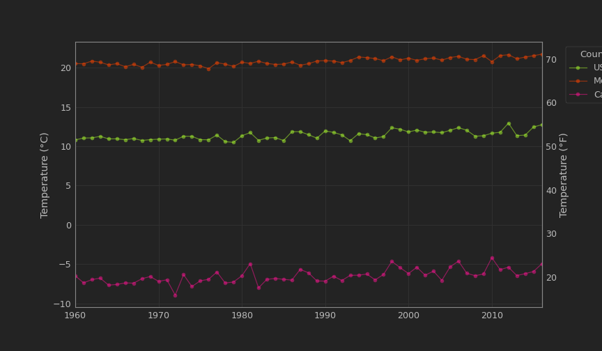
Canada it’s the country with more fluctuations. EUA had some too. Now, let’s plot the $CO_2$ emissions per country and also the value of $\Delta T$ per year.
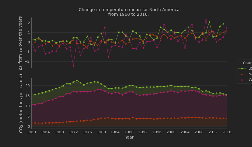
This gives us an idea of how important is the $CO_2$ emission for the entire enviroment. Canada had a significant increase of $\Delta T$ over the years. USA had the most fluctuating values for $\Delta T$ and it’s not a surprise, that country had a lot of $CO_2$ emissions, more that the other countries.
That’s all for this post! You can check the jupyter notebook from this problem here.